Generative AI has emerged as a strong and well-liked instrument to automate content material creation and easy duties. From personalized content material creation to supply code era, it might probably improve each our productiveness and inventive potential.
Companies need to leverage the facility of LLMs, like Gemini, however many could have safety considerations and need extra management round how workers make certain of those new instruments. For instance, corporations could need to be sure that numerous types of delicate information, comparable to Personally Identifiable Info (PII), monetary information and inside mental property, is to not be shared publicly on Generative AI platforms. Safety leaders face the problem of discovering the proper steadiness — enabling workers to leverage AI to spice up effectivity, whereas additionally safeguarding company information.
On this weblog submit, we’ll discover reporting and enforcement insurance policies that enterprise safety groups can implement inside Chrome Enterprise Premium for information loss prevention (DLP).
1. View login occasions* to know utilization of Generative AI providers inside the group. With Chrome Enterprise’s Reporting Connector, safety and IT groups can see when a consumer efficiently indicators into a particular area, together with Generative AI web sites. Safety Operations groups can additional leverage this telemetry to detect anomalies and threats by streaming the information into Chronicle or different third-party SIEMs at no extra value.
2. Allow URL Filtering to warn customers about delicate information insurance policies and allow them to determine whether or not or not they need to navigate to the URL, or to dam customers from navigating to sure teams of web sites altogether.
For instance, with Chrome Enterprise URL Filtering, IT admins can create guidelines that warn builders to not submit supply code to particular Generative AI apps or instruments, or block them.
3. Warn, block or monitor delicate information actions inside Generative AI web sites with dynamic content-based guidelines for actions like paste, file uploads/downloads, and print. Chrome Enterprise DLP guidelines give IT admins granular management over browser actions, comparable to coming into monetary info in Gen AI web sites. Admins can customise DLP guidelines to limit the kind and quantity of information entered into these web sites from managed browsers.
For many organizations, safely leveraging Generative AI requires a certain quantity of management. As enterprises work by means of their insurance policies and processes involving GenAI, Chrome Enterprise Premium empowers them to strike the steadiness that works finest. Hear straight from safety leaders at Snap on their use of DLP for Gen AI in this recording right here.
Be taught extra about how Chrome Enterprise can safe companies identical to yours right here.
Hundreds of organizations construct information integration pipelines to extract and remodel information. They set up information high quality guidelines to make sure the extracted information is of top quality for correct enterprise choices. These guidelines generally assess the info based mostly on mounted standards reflecting the present enterprise state. Nonetheless, when the enterprise surroundings adjustments, information properties shift, rendering these mounted standards outdated and inflicting poor information high quality.
For instance, an information engineer at a retail firm established a rule that validates every day gross sales should exceed a 1-million-dollar threshold. After a number of months, every day gross sales surpassed 2 million {dollars}, rendering the brink out of date. The info engineer couldn’t replace the foundations to mirror the newest thresholds as a consequence of lack of notification and the hassle required to manually analyze and replace the rule. Later within the month, enterprise customers observed a 25% drop of their gross sales. After hours of investigation, the info engineers found that an extract, remodel, and cargo (ETL) pipeline accountable for extracting information from some shops had failed with out producing errors. The rule with outdated thresholds continued to function efficiently with out detecting this anomaly.
Additionally, breaks or gaps that considerably deviate from the seasonal sample can typically level to information high quality points. As an illustration, retail gross sales could also be highest on weekends and vacation seasons whereas comparatively low on weekdays. Divergence from this sample could point out information high quality points reminiscent of lacking information from a retailer or shifts in enterprise circumstances. Knowledge high quality guidelines with mounted standards can’t detect seasonal patterns as a result of this requires superior algorithms that may study from previous patterns and seize seasonality to detect deviations. You want the flexibility spot anomalies with ease, enabling you to proactively detect information high quality points and make assured enterprise choices.
To handle these challenges, we’re excited to announce the overall availability of anomaly detection capabilities in AWS Glue Knowledge High quality. On this put up, we show how this characteristic works with an instance. We offer an AWS Cloud Formation template to deploy this setup and experiment with this characteristic.
For completeness and ease of navigation, you’ll be able to discover all the next AWS Glue Knowledge High quality weblog posts. It will enable you to perceive all the opposite capabilities of AWS Glue Knowledge High quality, along with anomaly detection.
Resolution overview
For our use case, an information engineer needs to measure and monitor information high quality of the New York taxi journey dataset. The info engineer is aware of about a number of guidelines, however needs to observe essential columns and be notified about any anomalies in these columns. These columns embrace fare quantity, and the info engineer needs to be notified about any main deviations. One other attribute is the variety of rides, which varies throughout peak hours, mid-day hours, and night time hours. Additionally, as town grows, there will probably be gradual enhance within the variety of rides total. We use anomaly detection to assist arrange and keep guidelines for this seasonality and rising pattern.
We show this characteristic with the next steps:
Deploy a CloudFormation template that may generate 7 days of NYC taxi information.
Create an AWS Glue ETL job and configure the anomaly detection functionality.
Run the job for six days and discover how AWS Glue Knowledge High quality learns from information statistics and detects anomalies.
Arrange assets with AWS CloudFormation
This put up features a CloudFormation template for a fast setup. You’ll be able to assessment and customise it to fit your wants. The template generates the next assets:
To create your assets, full the next steps:
Launch your CloudFormation stack in us-east-1.
Hold all settings as default.
Choose I acknowledge that AWS CloudFormation would possibly create IAM assets and select Create stack.
When the stack is full, copy the AWS Glue script to the S3 bucket anomaly-detection-blog--.
As a part of the CloudFormation template, an information generator AWS Glue job is provisioned in your AWS account. Full the next steps to run the job:
On the AWS Glue console, select ETL jobs within the navigation pane.
Select the job
Evaluation the script on the Script
On the Job particulars tab, confirm the job run parameters within the Superior part:
bucket_name – The S3 bucket title the place you need the info to be generated.
bucket_prefix – The prefix within the S3 bucket.
gluecatalog_database_name – The database title within the AWS Glue Knowledge Catalog that was created by the CloudFormation template.
gluecatalog_table_name – The desk title to be created within the Knowledge Catalog within the database.
Select Run to run this job.
On the Runs tab, monitor the job till the Run standing column exhibits as Succeeded.
When the job is full, it would have generated the NYC taxi dataset for the date vary of Could 1, 2024, to Could 7, 2024, within the specified S3 bucket and cataloged the desk and partitions within the Knowledge Catalog for 12 months, month, day, and hour. This dataset accommodates 7 day of hourly rides that fluctuates between excessive and low on alternate days. As an illustration, on Monday, there are roughly 1,400 rides, on Tuesday round 700 rides, and this sample continues. Of the 7 days, the primary 5 days of knowledge is non-anomalous. Nonetheless, on the sixth day, an anomaly happens the place the variety of rows jumps to round 2,200 and the fare_amount is about to an unusually excessive worth of 95 for mid-day site visitors.
Create an AWS Glue visible ETL job
Full the next steps:
On the AWS Glue console, create a brand new AWS Glue visible job named anomaly-detection-blog-visual.
On the Job particulars tab, present the IAM function created by the CloudFormation stack.
On the Visible tab, add an S3 node for the info supply.
Present the next parameters:
For Database, select anomaly_detection_blog_db.
For Desk, select nyctaxi_raw.
For Partition predicate, enter 12 months==2024 AND month==5 AND day==1.
Add the Consider Knowledge High quality remodel and add use the next rule for fare_amount:
Guidelines = [
    ColumnValues "fare_amount" between 1 and 100
]
As a result of we’re nonetheless making an attempt to grasp the statistics on this metric, we begin with a variety rule, and after a number of runs, we’ll analyze the outcomes and fine-tune as wanted.
Subsequent, we add two analyzers: one for RowCount and one other for distinct values of pulocationid.
On the Anomaly detection tab, select Add analyzer.
For Statistics, enter RowCount.
Add a second analyzer.
For Statistics, enter DistinctValuesCount and for Columns, enter pulocationid.
Your last ruleset ought to appear to be the next code:
Guidelines = [
    ColumnValues "fare_amount" between 1 and 100
]
Analyzers = [
DistinctValuesCount "pulocationid",
RowCount
]
Save the job.
Now we have now generated an artificial NYC taxi dataset and authored an AWS Glue visible ETL job to learn from this dataset and carry out evaluation with one rule and two analyzers.
Run and consider the visible ETL job
Earlier than we run the job, let’s have a look at how anomaly detection works. On this instance, we now have configured one rule and two analyzers. Guidelines have thresholds to match what attractiveness like. Generally, you would possibly know the essential columns, however not know particular thresholds. Guidelines and analyzers collect information statistics or information profiles. On this instance, AWS Glue Knowledge High quality will collect 4 statistics (a ColumnValue rule will collect two statistics, specifically minimal and most fare quantity, and two analyzers will collect two statistics). After gathering three information factors from three runs, AWS Glue Knowledge High quality will predict the fourth run together with higher and decrease bounds. It’s going to then evaluate the anticipated worth with the precise worth. When the precise worth breaches the anticipated higher or decrease bounds, it would create an anomaly.
Let’s see this in motion.
Run the job for five days and analyze outcomes
As a result of the primary 5 days of knowledge is non-anomalous, it would set a baseline with seasonality for coaching the mannequin. Full the next steps to run the job 5 occasions, as soon as for every day’s partition:
Select the S3 node on the Visible tab and go to its properties.
Set the day subject within the partition predicate to 1.
Select Run to run this job.
Monitor the job on the Runs tab for Succeeded
Repeat these steps 4 extra occasions, every time incrementing the day subject within the partition predicate. Run the roles at roughly common intervals to get a clear graph that simulates the automated scheduled pipeline.
After 5 profitable runs, go to the Knowledge high quality tab, the place it’s best to see the statistic gathered for fare_amount and RowCount.
The anomaly detection algorithm takes a minimal of three information factors to study and begin predicting. After three runs, you may even see a number of anomalies detected in your dataset. That is anticipated as a result of each new pattern is seen as an anomaly at first. Because the algorithm processes an increasing number of information, it learns from it and units the higher and decrease bounds in your information precisely. The higher and decrease sure predictions are depending on the interval between the job runs.
Additionally, we are able to observe that the info high quality rating is all the time 100% based mostly on the generic fare_amount rule we arrange. You’ll be able to discover the statistics by selecting the View traits hyperlinks for every of the metrics to deep dive into the values. For instance, the next screenshot exhibits the values for minimal fare_amount over a set of runs.
The mannequin has predicted the higher sure to be round 1.4 and the decrease sure to be round 1.2 for the minimal statistic of the fare_amount metric. When these bounds are breached, it will be thought of an anomaly.
Run the job for the sixth (anomalous) day and analyze outcomes
For the sixth day, we course of a file that has two identified anomalies. With this run, it’s best to see anomalies detected on the graph. Full the next steps:
Select the S3 node on the Visible tab and go to its properties.
Set the day subject within the partition predicate to 6.
Select Run to run this job.
Monitor the job on the Runs tab for Succeeded
It’s best to see a screenshot as follows the place two anomalies are detected as anticipated: one for fare_amount with a excessive worth of 95 and one for RowCount with a price of 2776.
Discover that despite the fact that the fare_amount rating was anomalous and excessive, the info high quality rating continues to be 100%. We’ll repair this later.
Let’s examine the RowCount anomaly additional. As proven within the following screenshot, in the event you develop the anomaly file, you’ll be able to see how the prediction higher sure was breached to trigger this anomaly.
Up till this level, we noticed how a baseline was set for the mannequin coaching and statistics collected. We additionally noticed how an anomalous worth in our dataset was flagged as an anomaly by the mannequin.
Replace information high quality guidelines based mostly on findings
Now that we perceive the statistics, lets alter our ruleset such that when the foundations fail, the info high quality rating is impacted. We take rule suggestions from the anomaly detection characteristic and add them to the ruleset.
As proven earlier, when the anomaly is detected, it provides you rule suggestions to the proper of the graph. For this case, the rule suggestion states the RowCount metric needs to be between 275.0–1966.0. Let’s replace our visible job.
Copy the rule below Rule Suggestions for RowCount.
On the Visible tab, select the Consider Knowledge High quality node, go to its properties, and enter the rule within the guidelines editor.
Repeat these steps for fare_amount.
You’ll be able to alter your last ruleset to look as follows:
Guidelines = [
    ColumnValues "fare_amount" <= 52,
    RowCount between 100 and 1800
]
Analyzers = [
DistinctValuesCount "pulocationid",
RowCount
]
Save the job, however don’t run it but.
To date, we now have discovered learn how to use statistics collected to regulate the foundations and ensure our information high quality rating is correct. However there’s a downside—the anomalous values affect the mannequin coaching, forcing the higher and decrease bounds to regulate to the anomaly. We have to exclude these information factors.
Exclude the RowCount anomaly
When an anomaly is detected in your dataset, the higher and decrease sure prediction will alter to it as a result of it would assume it’s a seasonality by default. After investigation, in the event you consider that it’s certainly an anomaly and never a seasonality, it’s best to exclude the anomaly so it doesn’t impression future predictions.
As a result of our sixth run is an anomaly, you’ll be able to full the next steps to exclude it:
On the Anomalies tab, choose the anomaly row you wish to exclude.
On the Edit coaching inputs menu, select Exclude anomaly.
Select Save and retrain.
Select the refresh icon.
If you must view earlier anomalous runs, navigate to the Knowledge high quality pattern graph, hover over the anomaly information level, and select View chosen run outcomes. It will take you to the job run on a brand new tab the place you’ll be able to comply with the previous steps to exclude the anomaly.
Alternatively, in the event you ran the job over a time period and have to exclude a number of information factors, you are able to do so from the Statistics tab:
On the Knowledge high quality tab, go to the Statistics tab and select View traits for RowCount.
Choose the worth you wish to exclude.
On the Edit coaching inputs menu, select Exclude anomaly.
Select Save and retrain.
Select the refresh icon.
It might take a number of seconds to mirror the change.
The next determine exhibits how the mannequin adjusted to the anomalies earlier than exclusion.
The next determine exhibits how the mannequin retrained itself after the anomalies have been excluded.
Now that the predictions are adjusted, all future out-of-range values will probably be detected as anomalies once more.
Now you’ll be able to run the job for day 7, which has non-anomalous information, and discover the traits.
Add an anomaly detection rule
It may be difficult to switch the rule values with the rising enterprise traits. For instance, in some unspecified time in the future in future, the NYC taxi rows will exceed the now anomalous RowCount worth of 2200. As you run the job over an extended time period, the mannequin matures and fine-tunes itself to the incoming information. At that time, you can also make anomaly detection a rule by itself so that you don’t should replace the values and may cease the roles or lower the info high quality rating. When there’s an anomaly within the dataset, it implies that the standard of the info just isn’t good and the info high quality rating ought to mirror that. Let’s add a DetectAnomalies rule for the RowCount metric.
On the Visible tab, select the Consider Knowledge High quality node.
For Rule varieties, seek for and select DetectAnomalies, then add the rule.
Your last ruleset ought to appear to be the next screenshot. Discover that you simply don’t have any values for RowCount.
That is the actual energy of anomaly detection in your ETL pipeline.
Seasonality use case
The next screenshot exhibits an instance of a pattern with a extra in-depth seasonality. The NYC taxi dataset has a various variety of rides all through the day relying on peak hours, mid-day hours, and night time hours. The next anomaly detection job ran on the present timestamp each hour to seize the seasonality of the day, and the higher and decrease bounds have adjusted to this seasonality. When the variety of rides drops unexpectedly inside that seasonality pattern, it’s detected as an anomaly.
We noticed how an information engineer can construct anomaly detection into their pipeline for the incoming move of knowledge being processed at common interval. We additionally discovered how one can make anomaly detection a rule after the mannequin is mature and fail the job, if an anomaly is detected, to keep away from redundant downstream processing.
Clear up
To wash up your assets, full the next steps:
On the Amazon S3 console, empty the S3 bucket created by the CloudFormation stack.
On the AWS Glue console, delete the anomaly-detection-blog-visual AWS Glue job you created.
When you deployed the CloudFormation stack, delete the stack on the AWS CloudFormation console.
Conclusion
This put up demonstrated the brand new anomaly detection characteristic in AWS Glue Knowledge High quality. Though information high quality static and dynamic guidelines are very helpful, they will’t seize information seasonality and the way information adjustments as your online business evolves. A machine studying mannequin supporting anomaly detection can perceive these advanced adjustments and inform you of anomalies within the dataset. Additionally, the suggestions offered can assist you writer correct information high quality guidelines. It’s also possible to allow anomaly detection as a rule after the mannequin has been skilled over an extended time period on a ample quantity of knowledge.
To study extra about AWS Glue Knowledge High quality, take a look at AWS Glue Knowledge High quality. If in case you have any feedback or suggestions, go away them within the feedback part.
Concerning the authors
Noah Soprala is a Options Architect based mostly out of Dallas. He’s a trusted advisor to his prospects within the ISV trade and helps them construct progressive options utilizing AWS applied sciences. Noah has over 20+ years of expertise in consulting, growth and resolution supply.
Shovan Kanjilal is a Senior Analytics and Machine Studying Architect with Amazon Internet Providers. He’s enthusiastic about serving to prospects construct scalable, safe and high-performance information options within the cloud.
Shiv Narayanan is a Technical Product Supervisor for AWS Glue’s information administration capabilities like information high quality, delicate information detection and streaming capabilities. Shiv has over 20 years of knowledge administration expertise in consulting, enterprise growth and product administration.
Jesus Max Hernandez is a Software program Growth Engineer at AWS Glue. He joined the workforce after graduating from The College of Texas at El Paso, and the vast majority of his work has been in frontend growth. Outdoors of labor, you will discover him practising guitar or taking part in flag soccer.
Tyler McDaniel is a software program growth engineer on the AWS Glue workforce with various technical pursuits, together with high-performance computing and optimization, distributed methods, and machine studying operations. He has eight years of expertise in software program and analysis roles.
Andrius Juodelis is a Software program Growth Engineer at AWS Glue with a eager curiosity in AI, designing machine studying methods, and information engineering.
A deepfake is an artificial media method that makes use of deep studying to create or manipulate video, audio, or pictures to current one thing that didn’t truly happen. Deepfakes have gained consideration partly on account of their potential for misuse, similar to creating cast movies for political manipulation or spreading misinformation.
Ryan Ofman is a Lead Engineer and Head of Science Communication at DeepMedia, which is a platform for AI-powered deepfake detection. He joins the present to speak in regards to the state of deepfakes, their origin, and the right way to detect them.
Sean’s been a tutorial, startup founder, and Googler. He has printed works masking a variety of matters from data visualization to quantum computing. At the moment, Sean is Head of Advertising and marketing and Developer Relations at Skyflow and host of the podcast Partially Redacted, a podcast about privateness and safety engineering. You possibly can join with Sean on Twitter @seanfalconer .
WorkOS is a contemporary id platform constructed for B2B SaaS, offering a faster path to land enterprise offers.
It offers versatile APIs for authentication, consumer id, and complicated options like SSO and SCIM provisioning.
It’s a drop-in substitute for Auth0 (auth-zero) and helps as much as 1 million month-to-month energetic customers without spending a dime. As we speak, a whole lot of high-growth scale-ups are already powered by WorkOS, together with ones you in all probability know, like Vercel, Webflow, Perplexity, and Drata.
Not too long ago, WorkOS introduced the acquisition of Warrant, the Nice Grained Authorization service. Warrant’s product is predicated on a groundbreaking authorization system known as Zanzibar, which was initially designed by Google to energy Google Docs and YouTube. This permits quick authorization checks at huge scale whereas sustaining a versatile mannequin that may be tailored to even essentially the most complicated use instances.
If you’re at present seeking to construct Function-Primarily based Entry Management or different enterprise options like SAML , SCIM, or consumer administration, try workos.com/SED to get began without spending a dime.
This episode of Software program Engineering Day by day is delivered to you by Vantage. Have you learnt what your cloud invoice shall be for this month?
For a lot of corporations, cloud prices are the quantity two line merchandise of their price range and the primary quickest rising class of spend.
Vantage helps you get a deal with in your cloud payments, with self-serve studies and dashboards constructed for engineers, finance, and operations groups. With Vantage, you may put prices within the fingers of the service house owners and managers who generate them—giving them budgets, alerts, anomaly detection, and granular visibility into each greenback.
With native billing integrations with dozens of cloud providers, together with AWS, Azure, GCP, Datadog, Snowflake, and Kubernetes, Vantage is the one FinOps platform to observe and scale back all of your cloud payments.
To get began, head to vantage.sh, join your accounts, and get a free financial savings estimate as a part of a 14-day free trial.
Bored with stitching AWS providers collectively when you may be constructing options to your customers?
With Convex, you get a contemporary backend as a service: a versatile 100% ACID-compliant database, pure TypeScript cloud capabilities, end-to-end sort security along with your app, deep React integration, and ubiquitous real-time updates. Every thing you should construct your full stack venture sooner than ever, and no glue required. Get began on Convex without spending a dime in the present day!
Observe: Like a number of prior ones, this publish is an excerpt from the forthcoming e-book, Deep Studying and Scientific Computing with R torch. And like many excerpts, it’s a product of laborious trade-offs. For extra depth and extra examples, I’ve to ask you to please seek the advice of the e-book.
Wavelets and the Wavelet Remodel
What are wavelets? Just like the Fourier foundation, they’re capabilities; however they don’t prolong infinitely. As an alternative, they’re localized in time: Away from the middle, they shortly decay to zero. Along with a location parameter, in addition they have a scale: At completely different scales, they seem squished or stretched. Squished, they’ll do higher at detecting excessive frequencies; the converse applies once they’re stretched out in time.
The essential operation concerned within the Wavelet Remodel is convolution – have the (flipped) wavelet slide over the info, computing a sequence of dot merchandise. This manner, the wavelet is principally searching for similarity.
As to the wavelet capabilities themselves, there are various of them. In a sensible software, we’d wish to experiment and decide the one which works finest for the given knowledge. In comparison with the DFT and spectrograms, extra experimentation tends to be concerned in wavelet evaluation.
The subject of wavelets could be very completely different from that of Fourier transforms in different respects, as effectively. Notably, there’s a lot much less standardization in terminology, use of symbols, and precise practices. On this introduction, I’m leaning closely on one particular exposition, the one in Arnt Vistnes’ very good e-book on waves (Vistnes 2018). In different phrases, each terminology and examples mirror the alternatives made in that e-book.
Introducing the Morlet wavelet
The Morlet, also called Gabor, wavelet is outlined like so:
This formulation pertains to discretized knowledge, the sorts of information we work with in observe. Thus, (t_k) and (t_n) designate deadlines, or equivalently, particular person time-series samples.
This equation seems daunting at first, however we will “tame” it a bit by analyzing its construction, and pointing to the principle actors. For concreteness, although, we first take a look at an instance wavelet.
We begin by implementing the above equation:
Evaluating code and mathematical formulation, we discover a distinction. The operate itself takes one argument, (t_n); its realization, 4 (omega, Ok, t_k, and t). It’s because the torch code is vectorized: On the one hand, omega, Ok, and t_k, which, within the method, correspond to (omega_{a}), (Ok), and (t_k) , are scalars. (Within the equation, they’re assumed to be mounted.) t, however, is a vector; it can maintain the measurement occasions of the sequence to be analyzed.
We decide instance values for omega, Ok, and t_k, in addition to a spread of occasions to guage the wavelet on, and plot its values:
What we see here’s a complicated sine curve – be aware the actual and imaginary elements, separated by a section shift of (pi/2) – that decays on either side of the middle. Trying again on the equation, we will determine the elements chargeable for each options. The primary time period within the equation, (e^{-i omega_{a} (t_n – t_k)}), generates the oscillation; the third, (e^{- omega_a^2 (t_n – t_k )^2 /(2K )^2}), causes the exponential decay away from the middle. (In case you’re questioning in regards to the second time period, (e^{-Ok^2}): For given (Ok), it’s only a fixed.)
The third time period truly is a Gaussian, with location parameter (t_k) and scale (Ok). We’ll discuss (Ok) in nice element quickly, however what’s with (t_k)? (t_k) is the middle of the wavelet; for the Morlet wavelet, that is additionally the situation of most amplitude. As distance from the middle will increase, values shortly method zero. That is what is supposed by wavelets being localized: They’re “energetic” solely on a brief vary of time.
The roles of (Ok) and (omega_a)
Now, we already mentioned that (Ok) is the size of the Gaussian; it thus determines how far the curve spreads out in time. However there may be additionally (omega_a). Trying again on the Gaussian time period, it, too, will affect the unfold.
First although, what’s (omega_a)? The subscript (a) stands for “evaluation”; thus, (omega_a) denotes a single frequency being probed.
Now, let’s first examine visually the respective impacts of (omega_a) and (Ok).
Morlet wavelet: Results of various scale and evaluation frequency.
Within the left column, we maintain (omega_a) fixed, and range (Ok). On the fitting, (omega_a) adjustments, and (Ok) stays the identical.
Firstly, we observe that the upper (Ok), the extra the curve will get unfold out. In a wavelet evaluation, which means that extra deadlines will contribute to the remodel’s output, leading to excessive precision as to frequency content material, however lack of decision in time. (We’ll return to this – central – trade-off quickly.)
As to (omega_a), its affect is twofold. On the one hand, within the Gaussian time period, it counteracts – precisely, even – the size parameter, (Ok). On the opposite, it determines the frequency, or equivalently, the interval, of the wave. To see this, check out the fitting column. Similar to the completely different frequencies, we have now, within the interval between 4 and 6, 4, six, or eight peaks, respectively.
This double function of (omega_a) is the explanation why, all-in-all, it does make a distinction whether or not we shrink (Ok), retaining (omega_a) fixed, or enhance (omega_a), holding (Ok) mounted.
This state of issues sounds sophisticated, however is much less problematic than it might sound. In observe, understanding the function of (Ok) is vital, since we have to decide wise (Ok) values to strive. As to the (omega_a), however, there will likely be a large number of them, equivalent to the vary of frequencies we analyze.
So we will perceive the affect of (Ok) in additional element, we have to take a primary take a look at the Wavelet Remodel.
Wavelet Remodel: An easy implementation
Whereas total, the subject of wavelets is extra multifaceted, and thus, could appear extra enigmatic than Fourier evaluation, the remodel itself is simpler to understand. It’s a sequence of native convolutions between wavelet and sign. Right here is the method for particular scale parameter (Ok), evaluation frequency (omega_a), and wavelet location (t_k):
That is only a dot product, computed between sign and complex-conjugated wavelet. (Right here complicated conjugation flips the wavelet in time, making this convolution, not correlation – a indisputable fact that issues so much, as you’ll see quickly.)
Correspondingly, easy implementation leads to a sequence of dot merchandise, every equivalent to a unique alignment of wavelet and sign. Beneath, in wavelet_transform(), arguments omega and Ok are scalars, whereas x, the sign, is a vector. The result’s the wavelet-transformed sign, for some particular Ok and omega of curiosity.
wavelet_transform<-operate(x, omega, Ok){n_samples<-dim(x)[1]W<-torch_complex(torch_zeros(n_samples), torch_zeros(n_samples))for(iin1:n_samples){# transfer heart of wavelett_k<-x[i, 1]m<-morlet(omega, Ok, t_k, x[, 1])# compute native dot product# be aware wavelet is conjugateddot<-torch_matmul(m$conj()$unsqueeze(1),x[, 2]$to(dtype =torch_cfloat()))W[i]<-dot}W}
To check this, we generate a easy sine wave that has a frequency of 100 Hertz in its first half, and double that within the second.
gencos<-operate(amp, freq, section, fs, period){x<-torch_arange(0, period, 1/fs)[1:-2]$unsqueeze(2)y<-amp*torch_cos(2*pi*freq*x+section)torch_cat(record(x, y), dim =2)}# sampling frequencyfs<-8000f1<-100f2<-200section<-0period<-0.25s1<-gencos(1, f1, section, fs, period)s2<-gencos(1, f2, section, fs, period)s3<-torch_cat(record(s1, s2), dim =1)s3[(dim(s1)[1]+1):(dim(s1)[1]*2), 1]<-s3[(dim(s1)[1]+1):(dim(s1)[1]*2), 1]+perioddf<-knowledge.body( x =as.numeric(s3[, 1]), y =as.numeric(s3[, 2]))ggplot(df, aes(x =x, y =y))+geom_line()+xlab("time")+ylab("amplitude")+theme_minimal()
An instance sign, consisting of a low-frequency and a high-frequency half.
Now, we run the Wavelet Remodel on this sign, for an evaluation frequency of 100 Hertz, and with a Ok parameter of two, discovered via fast experimentation:
Ok<-2omega<-2*pi*f1res<-wavelet_transform(x =s3, omega, Ok)df<-knowledge.body( x =as.numeric(s3[, 1]), y =as.numeric(res$abs()))ggplot(df, aes(x =x, y =y))+geom_line()+xlab("time")+ylab("Wavelet Remodel")+theme_minimal()
Wavelet Remodel of the above two-part sign. Evaluation frequency is 100 Hertz.
The remodel appropriately picks out the a part of the sign that matches the evaluation frequency. In the event you really feel like, you may wish to double-check what occurs for an evaluation frequency of 200 Hertz.
Now, in actuality we’ll wish to run this evaluation not for a single frequency, however a spread of frequencies we’re enthusiastic about. And we’ll wish to strive completely different scales Ok. Now, for those who executed the code above, you is perhaps fearful that this might take a lot of time.
Effectively, it by necessity takes longer to compute than its Fourier analogue, the spectrogram. For one, that’s as a result of with spectrograms, the evaluation is “simply” two-dimensional, the axes being time and frequency. With wavelets there are, as well as, completely different scales to be explored. And secondly, spectrograms function on complete home windows (with configurable overlap); a wavelet, however, slides over the sign in unit steps.
Nonetheless, the state of affairs will not be as grave because it sounds. The Wavelet Remodel being a convolution, we will implement it within the Fourier area as a substitute. We’ll try this very quickly, however first, as promised, let’s revisit the subject of various Ok.
Decision in time versus in frequency
We already noticed that the upper Ok, the extra spread-out the wavelet. We will use our first, maximally easy, instance, to analyze one rapid consequence. What, for instance, occurs for Ok set to twenty?
Ok<-20res<-wavelet_transform(x =s3, omega, Ok)df<-knowledge.body( x =as.numeric(s3[, 1]), y =as.numeric(res$abs()))ggplot(df, aes(x =x, y =y))+geom_line()+xlab("time")+ylab("Wavelet Remodel")+theme_minimal()
Wavelet Remodel of the above two-part sign, with Ok set to twenty as a substitute of two.
The Wavelet Remodel nonetheless picks out the proper area of the sign – however now, as a substitute of a rectangle-like consequence, we get a considerably smoothed model that doesn’t sharply separate the 2 areas.
Notably, the primary 0.05 seconds, too, present appreciable smoothing. The bigger a wavelet, the extra element-wise merchandise will likely be misplaced on the finish and the start. It’s because transforms are computed aligning the wavelet in any respect sign positions, from the very first to the final. Concretely, after we compute the dot product at location t_k = 1, only a single pattern of the sign is taken into account.
Aside from presumably introducing unreliability on the boundaries, how does wavelet scale have an effect on the evaluation? Effectively, since we’re correlating (convolving, technically; however on this case, the impact, ultimately, is similar) the wavelet with the sign, point-wise similarity is what issues. Concretely, assume the sign is a pure sine wave, the wavelet we’re utilizing is a windowed sinusoid just like the Morlet, and that we’ve discovered an optimum Ok that properly captures the sign’s frequency. Then another Ok, be it bigger or smaller, will lead to much less point-wise overlap.
Performing the Wavelet Remodel within the Fourier area
Quickly, we’ll run the Wavelet Remodel on an extended sign. Thus, it’s time to velocity up computation. We already mentioned that right here, we profit from time-domain convolution being equal to multiplication within the Fourier area. The general course of then is that this: First, compute the DFT of each sign and wavelet; second, multiply the outcomes; third, inverse-transform again to the time area.
The DFT of the sign is shortly computed:
F<-torch_fft_fft(s3[ , 2])
With the Morlet wavelet, we don’t even should run the FFT: Its Fourier-domain illustration might be said in closed kind. We’ll simply make use of that formulation from the outset. Right here it’s:
Evaluating this assertion of the wavelet to the time-domain one, we see that – as anticipated – as a substitute of parameters t and t_k it now takes omega and omega_a. The latter, omega_a, is the evaluation frequency, the one we’re probing for, a scalar; the previous, omega, the vary of frequencies that seem within the DFT of the sign.
In instantiating the wavelet, there may be one factor we have to pay particular consideration to. In FFT-think, the frequencies are bins; their quantity is set by the size of the sign (a size that, for its half, instantly relies on sampling frequency). Our wavelet, however, works with frequencies in Hertz (properly, from a person’s perspective; since this unit is significant to us). What this implies is that to morlet_fourier, as omega_a we have to cross not the worth in Hertz, however the corresponding FFT bin. Conversion is completed relating the variety of bins, dim(x)[1], to the sampling frequency of the sign, fs:
# once more search for 100Hz elementsomega<-2*pi*f1# want the bin equivalent to some frequency in Hzomega_bin<-f1/fs*dim(s3)[1]
We instantiate the wavelet, carry out the Fourier-domain multiplication, and inverse-transform the consequence:
Placing collectively wavelet instantiation and the steps concerned within the evaluation, we have now the next. (Observe tips on how to wavelet_transform_fourier, we now, conveniently, cross within the frequency worth in Hertz.)
We’ve already made vital progress. We’re prepared for the ultimate step: automating evaluation over a spread of frequencies of curiosity. It will lead to a three-dimensional illustration, the wavelet diagram.
Creating the wavelet diagram
Within the Fourier Remodel, the variety of coefficients we acquire relies on sign size, and successfully reduces to half the sampling frequency. With its wavelet analogue, since anyway we’re doing a loop over frequencies, we’d as effectively resolve which frequencies to research.
Firstly, the vary of frequencies of curiosity might be decided operating the DFT. The following query, then, is about granularity. Right here, I’ll be following the advice given in Vistnes’ e-book, which is predicated on the relation between present frequency worth and wavelet scale, Ok.
Iteration over frequencies is then carried out as a loop:
wavelet_grid<-operate(x, Ok, f_start, f_end, fs){# downsample evaluation frequency vary# as per Vistnes, eq. 14.17num_freqs<-1+log(f_end/f_start)/log(1+1/(8*Ok))freqs<-seq(f_start, f_end, size.out =ground(num_freqs))reworked<-torch_zeros(num_freqs, dim(x)[1], dtype =torch_cfloat())for(iin1:num_freqs){w<-wavelet_transform_fourier(x, freqs[i], Ok, fs)reworked[i, ]<-w}record(reworked, freqs)}
Calling wavelet_grid() will give us the evaluation frequencies used, along with the respective outputs from the Wavelet Remodel.
Subsequent, we create a utility operate that visualizes the consequence. By default, plot_wavelet_diagram() shows the magnitude of the wavelet-transformed sequence; it may well, nonetheless, plot the squared magnitudes, too, in addition to their sq. root, a technique a lot really useful by Vistnes whose effectiveness we’ll quickly have alternative to witness.
The operate deserves a couple of additional feedback.
Firstly, identical as we did with the evaluation frequencies, we down-sample the sign itself, avoiding to counsel a decision that isn’t truly current. The method, once more, is taken from Vistnes’ e-book.
Then, we use interpolation to acquire a brand new time-frequency grid. This step might even be needed if we maintain the unique grid, since when distances between grid factors are very small, R’s picture() might refuse to just accept axes as evenly spaced.
Lastly, be aware how frequencies are organized on a log scale. This results in rather more helpful visualizations.
plot_wavelet_diagram<-operate(x,freqs,grid,Ok,fs,f_end,sort="magnitude"){grid<-change(sort, magnitude =grid$abs(), magnitude_squared =torch_square(grid$abs()), magnitude_sqrt =torch_sqrt(grid$abs()))# downsample time sequence# as per Vistnes, eq. 14.9new_x_take_every<-max(Ok/24*fs/f_end, 1)new_x_length<-ground(dim(grid)[2]/new_x_take_every)new_x<-torch_arange(x[1],x[dim(x)[1]], step =x[dim(x)[1]]/new_x_length)# interpolate gridnew_grid<-nnf_interpolate(grid$view(c(1, 1, dim(grid)[1], dim(grid)[2])),c(dim(grid)[1], new_x_length))$squeeze()out<-as.matrix(new_grid)# plot log frequenciesfreqs<-log10(freqs)picture( x =as.numeric(new_x), y =freqs, z =t(out), ylab ="log frequency [Hz]", xlab ="time [s]", col =hcl.colours(12, palette ="Gentle grays"))foremost<-paste0("Wavelet Remodel, Ok = ", Ok)sub<-change(sort, magnitude ="Magnitude", magnitude_squared ="Magnitude squared", magnitude_sqrt ="Magnitude (sq. root)")mtext(aspect =3, line =2, at =0, adj =0, cex =1.3, foremost)mtext(aspect =3, line =1, at =0, adj =0, cex =1, sub)}
Let’s use this on a real-world instance.
An actual-world instance: Chaffinch’s music
For the case examine, I’ve chosen what, to me, was probably the most spectacular wavelet evaluation proven in Vistnes’ e-book. It’s a pattern of a chaffinch’s singing, and it’s out there on Vistnes’ web site.
We use torchaudio to load the file, and convert from stereo to mono utilizing tuneR’s appropriately named mono(). (For the sort of evaluation we’re doing, there isn’t a level in retaining two channels round.)
How does this look within the time area? (Don’t miss out on the event to truly hear to it, in your laptop computer.)
df<-knowledge.body(x =1:dim(x)[1], y =as.numeric(x))ggplot(df, aes(x =x, y =y))+geom_line()+xlab("pattern")+ylab("amplitude")+theme_minimal()
Chaffinch’s music.
Now, we have to decide an inexpensive vary of study frequencies. To that finish, we run the FFT:
On the x-axis, we plot frequencies, not pattern numbers, and for higher visibility, we zoom in a bit.
bins<-1:dim(F)[1]freqs<-bins/N*fs# the bin, not the frequencycutoff<-N/4df<-knowledge.body( x =freqs[1:cutoff], y =as.numeric(F$abs())[1:cutoff])ggplot(df, aes(x =x, y =y))+geom_col()+xlab("frequency (Hz)")+ylab("magnitude")+theme_minimal()
Chaffinch’s music, Fourier spectrum (excerpt).
Primarily based on this distribution, we will safely prohibit the vary of study frequencies to between, roughly, 1800 and 8500 Hertz. (That is additionally the vary really useful by Vistnes.)
First, although, let’s anchor expectations by making a spectrogram for this sign. Appropriate values for FFT dimension and window dimension had been discovered experimentally. And although, in spectrograms, you don’t see this performed typically, I discovered that displaying sq. roots of coefficient magnitudes yielded probably the most informative output.
fft_size<-1024window_size<-1024energy<-0.5spectrogram<-transform_spectrogram( n_fft =fft_size, win_length =window_size, normalized =TRUE, energy =energy)spec<-spectrogram(x)dim(spec)
[1] 513 257
Like we do with wavelet diagrams, we plot frequencies on a log scale.
bins<-1:dim(spec)[1]freqs<-bins*fs/fft_sizelog_freqs<-log10(freqs)frames<-1:(dim(spec)[2])seconds<-(frames/dim(spec)[2])*(dim(x)[1]/fs)picture(x =seconds, y =log_freqs, z =t(as.matrix(spec)), ylab ='log frequency [Hz]', xlab ='time [s]', col =hcl.colours(12, palette ="Gentle grays"))foremost<-paste0("Spectrogram, window dimension = ", window_size)sub<-"Magnitude (sq. root)"mtext(aspect =3, line =2, at =0, adj =0, cex =1.3, foremost)mtext(aspect =3, line =1, at =0, adj =0, cex =1, sub)
Chaffinch’s music, spectrogram.
The spectrogram already exhibits a particular sample. Let’s see what might be performed with wavelet evaluation. Having experimented with a couple of completely different Ok, I agree with Vistnes that Ok = 48 makes for a superb selection:
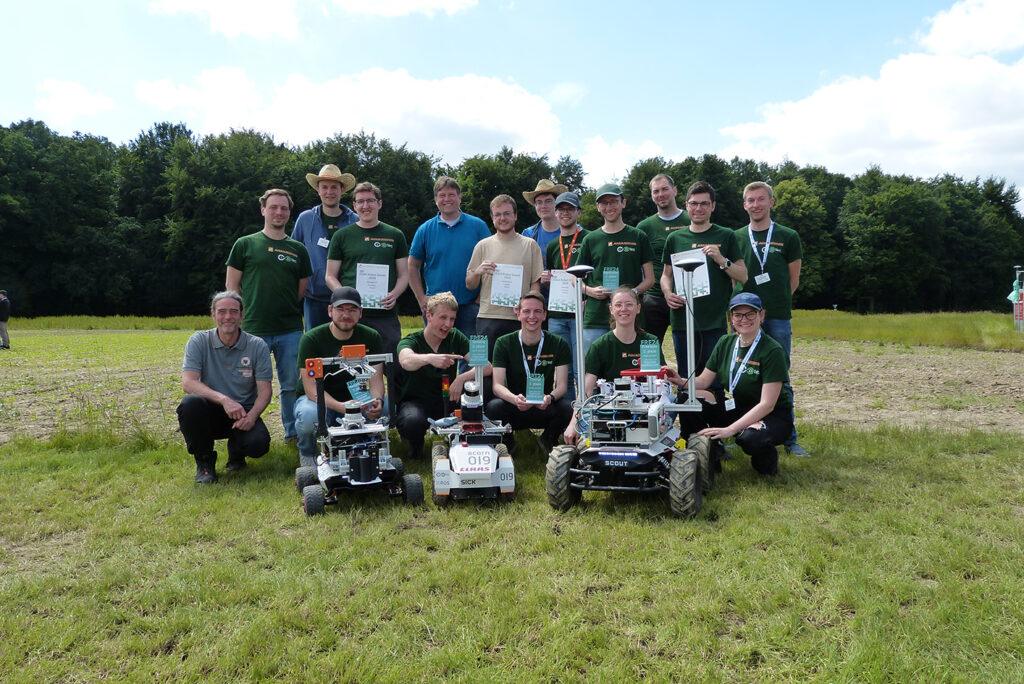
Studentisches Staff der Hochschule Osnabrück und der Universität Osnabrück erzielt herausragenden Erfolg beim Internationalen Feldroboter-Wettbewerb und stellt Kompetenz, Innovationskraft und Teamgeist unter Beweis
Foto: Hochschule Osnabrück (Andreas Linz)
(lifePR) (Osnabrück, 23.08.2024) Das studentische Staff der Hochschule Osnabrück und der Universität Osnabrück hat beim diesjährigen Internationalen Feldroboter-Wettbewerb einen bemerkenswerten Erfolg erzielt. Das Staff sicherte sich eine Gold- und vier Bronzemedaillen und bewies damit erneut Osnabrücks herausragende Kompetenz in der Feldrobotik.
Feldroboter-Wettbewerb: traditionell innovativ
Das traditionsreiche Occasion fand bereits zum 21. Mal statt – in diesem Jahr während der Feldtage der Deutschen Landwirtschafts-Gesellschaft (DLG) auf Intestine Brockhof in Erwitte. Studierende – diesmal waren es zwölf Groups aus fünf europäischen Ländern – messen sich dabei in verschiedenen Disziplinen. Beim Bauen und Programmieren ihrer Feldroboter greifen sie auf neueste Technologien zurück und lernen, fachübergreifend und zielorientiert zusammenzuarbeiten.
Osnabrücker Staff Acorn
Das Staff Acorn bestand aus 17 Studierenden der Hochschule Osnabrück und der Universität Osnabrück. Unter der Leitung von den Kapitänen Philipp Gehricke ({Hardware}) und Justus Braun (Software program) arbeiteten die Teammitglieder aus den Studiengängen der Informatik, Cognitive Science und Mechatronic Programs Engineering eng zusammen. Sie wurden mit einem beeindruckenden dritten Platz in der Gesamtwertung belohnt – hinter den Groups FREDT aus Braunschweig und Carbonite vom Schülerforschungszentrum Überlingen, die sich den ersten Platz geteilt haben. Unterstützt wurde das Osnabrücker Staff von den wissenschaftlichen Mitarbeitern Andreas Linz (Hochschule Osnabrück) sowie Alexander Mock und Isaak Ihorst (Universität Osnabrück). Wichtige Sponsoren wie AMAZONEN-WERKE H. DREYER SE & Co. KG, CLAAS KGaA mbH, iotec GmbH und Allied Imaginative and prescient Applied sciences GmbH trugen ebenfalls zum Erfolg des Groups bei.
Goldmedaille für klassischen Ansatz in mobiler Robotik
In einer der anspruchsvollsten Aufgaben des Wettbewerbs ging es darum, bereits kartierte Pflanzen präzise anzufahren und zu behandeln. Hier überzeugte der Roboter des Groups Acorn mit einem außergewöhnlich hohen Grad an Autonomie. Trotz des Verbots von GPS konnte der Roboter die vorgegebenen Punkte präzise anfahren. „Wir haben dafür eine Technologie verwendet, die sonst in der klassischen Indoor-Robotik, additionally in Innenräumen, für die Pfadplanung und Ausführung eingesetzt wird“, erklärt Justus Braun. Philipp Gehricke ergänzt: „Für die Blumenbehandlung haben wir eine spezielle Vorrichtung konstruiert, um die punktgenau Schiedsrichterspray sprühen zu können.“ Ein anschließender Take a look at zeigte zudem, dass der Osnabrücker Roboter über Stunden hinweg komplett eigenständig arbeiten konnte und sich sogar an verändernde Bedingungen anpasste – etwa Menschenbewegungen auf dem Feld. Die Leistung des Groups überzeugte die internationale Fachjury und führte schließlich zur verdienten Goldmedaille.
Vier Bronzemedaillen in verschiedenen Kategorien
Neben der Goldmedaille konnte das Staff Acorn in mehreren weiteren Aufgaben überzeugen und sicherte sich insgesamt vier Bronzemedaillen in den Kategorien „Navigation durch Maisreihen“, „Finden und Kartieren von Blumen“, „Freistil“ sowie in der Gesamtwertung des Wettbewerbs. So navigierte Acorn erfolgreich durch vier Maisreihen, ohne eine einzige Pflanze zu beschädigen. Entscheidend waren dafür neben einer intelligenten Konstruktion auch eine durchdachte Software program, die Höhenunterschiede auf dem Feld analysierte und daraus die Befahrbarkeit einzelner Strecken berechnete. Beim Finden und Kartieren von Blumen untersuchte der Roboter des Osnabrücker Groups die meiste Fläche des Spielfelds und erkannte auch die meisten Blumen. Für die Bilderkennung hat das Staff Künstliche Intelligenz eingesetzt. Abzüge aufgrund von Ungenauigkeiten führten hier zu Platz drei. Im Freistil-Wettbewerb stellte das Staff eine Lösung für präzises Säen vor: Eine Drohne erkannte fehlenden Rasen und der Roboter verteilte selbständig Rasensamen auf den kahlen Stellen.
Moderne Technologien für nachhaltige Landwirtschaft
Das Betreuerteam freut sich über den beeindruckenden Erfolg der Osnabrücker Studierenden: „Ein Platz auf dem Siegertreppchen bei einem anspruchsvollen internationalen Wettbewerb unterstreicht die hohe Kompetenz und Innovationskraft unserer beiden Hochschulen im Bereich der Robotik“, so Andreas Linz. Sein Kollege Alexander Mock betont: „Damit setzt das studentische Staff Maßstäbe für zukünftige Wettbewerbe. Es nutzt bestehende und entwickelt neue Technologien, die das Potenzial haben, die Landwirtschaft nachhaltig zu verändern.“
Zum Hintergrund:
Dem Staff Acorn gehören Studierende der Hochschule Osnabrück und der Universität Osnabrück an:
Justus Braun (Kapitän Software program), Philipp Gehricke (Kapitän {Hardware}), Marco Tassemeier, Simon Balzer, Marc Meijer, Christopher Sieh, Piper Powell, Can-Leon Petermöller, Andreas Klaas, Lena Brüggemann, Lara Lüking, Jannik Jose, Leon Rabius, Thorben Boße, Ole Georg Oevermann, Until Stückemann und Gerrit Lange.
Veranstalter des Subject Robotic Occasions 2024 waren:
Die Hochschule Osnabrück mit Prof. Dr. Stefan Stiene, Silke Becker und Andreas Linz
Die Technische Hochschule Ostwestfalen-Lippe mit Prof. Dr. Burkhard Wrenger und Carsten Langohr
Agrotech Valley Discussion board e. V. mit Geschäftsführer Robert Everwand, Francisca Wesner und Karen Sommer

.png)


 Noah Soprala is a Options Architect based mostly out of Dallas. He’s a trusted advisor to his prospects within the ISV trade and helps them construct progressive options utilizing AWS applied sciences. Noah has over 20+ years of expertise in consulting, growth and resolution supply.
 Shovan Kanjilal is a Senior Analytics and Machine Studying Architect with Amazon Internet Providers. He’s enthusiastic about serving to prospects construct scalable, safe and high-performance information options within the cloud.
 Shiv Narayanan is a Technical Product Supervisor for AWS Glue’s information administration capabilities like information high quality, delicate information detection and streaming capabilities. Shiv has over 20 years of knowledge administration expertise in consulting, enterprise growth and product administration.
 Jesus Max Hernandez is a Software program Growth Engineer at AWS Glue. He joined the workforce after graduating from The College of Texas at El Paso, and the vast majority of his work has been in frontend growth. Outdoors of labor, you will discover him practising guitar or taking part in flag soccer.
 Tyler McDaniel is a software program growth engineer on the AWS Glue workforce with various technical pursuits, together with high-performance computing and optimization, distributed methods, and machine studying operations. He has eight years of expertise in software program and analysis roles.
 Andrius Juodelis is a Software program Growth Engineer at AWS Glue with a eager curiosity in AI, designing machine studying methods, and information engineering.