
YOLO fashions have made vital contributions to laptop imaginative and prescient in varied functions, equivalent to object detection, segmentation, pose estimation, automobile velocity detection, and multimodal duties. Whereas understanding their functions is essential, it’s equally necessary to know the way these fashions are constructed and the way they work. This text will concentrate on that side.
On this article, we can be constructing the newest object detection mannequin, Yolov11 from scratch in Pytorch. In case you are new to YOLOv11, I might strongly suggest studying A Complete Information to YOLOv11 Object Detection.
Studying Goals
- Perceive the structure and key parts of YOLOv11 for superior object detection.
- Learn the way YOLOv11 handles multi-task studying for object detection, segmentation, and classification.
- Discover the function of YOLOv11’s spine and neck in enhancing mannequin efficiency.
- Look at the sensible functions of YOLOv11 in real-world AI initiatives.
- Uncover how YOLOv11 optimizes effectivity for deployment in each edge and cloud environments.
This text was printed as part of the Knowledge Science Blogathon.
What are YOLO Fashions?
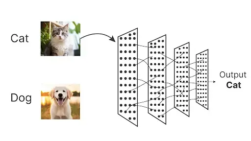
YOLO (You Solely Look As soon as) fashions are identified for his or her effectivity and reliability in object detection duties. They provide an awesome steadiness of small mannequin sizes, excessive accuracy, and spectacular imply Common Precision (mAP) scores. The structure of YOLO fashions performs a key function of their success, with optimized pipelines for real-time detection and minimal computational overhead. Over time, varied YOLO variations have been launched, every introducing improvements to enhance efficiency, scale back latency, and develop utility areas.
The YOLO household has developed considerably from its unique model, with every iteration—YOLOv2, YOLOv3, and past—providing enhancements in detection accuracy, velocity, and have extraction. Variations like YOLOv4 and YOLOv5 launched architectural developments, together with CSPNet and mosaic augmentation, enhancing efficiency. The later fashions, YOLOv6 to YOLOv8, targeted on creating light-weight architectures preferrred for edge machine deployment whereas sustaining excessive efficiency. YOLOv11, nonetheless, takes a special strategy, focusing extra on sensible functions than conventional analysis, with Ultralytics emphasizing real-world options over tutorial documentation, signaling a shift in direction of application-driven improvement.
Ultralytics has not printed a proper analysis paper for YOLO11 because of the quickly evolving nature of the fashions. We concentrate on advancing the expertise and making it simpler to make use of, somewhat than producing static documentation. Supply
The accompanying desk offers a complete overview of the assorted YOLO variations, mapping their parameters to corresponding mAP scores, providing precious insights into their comparative efficiency.
| Mannequin | Measurement (pixels) | mAPval | Velocity (CPU ONNX) | Velocity (T4 TensorRT10) | Params (M) | FLOPs (B) |
|---|---|---|---|---|---|---|
| YOLOv11n | 640 | 39.5 | 56.1 ± 0.8 | 1.5 ± 0.0 | 2.6 | 6.5 |
| YOLOv11s | 640 | 47.0 | 90.0 ± 1.2 | 2.5 ± 0.0 | 9.4 | 21.5 |
| YOLOv11m | 640 | 51.5 | 183.2 ± 2.0 | 4.7 ± 0.1 | 20.1 | 68.0 |
| YOLOv11 | 640 | 53.4 | 238.6 ± 1.4 | 6.2 ± 0.1 | 25.3 | 86.9 |
| YOLOv11x | 640 | 54.7 | 462.8 ± 6.7 | 11.3 ± 0.2 | 56.9 | 194.9 |
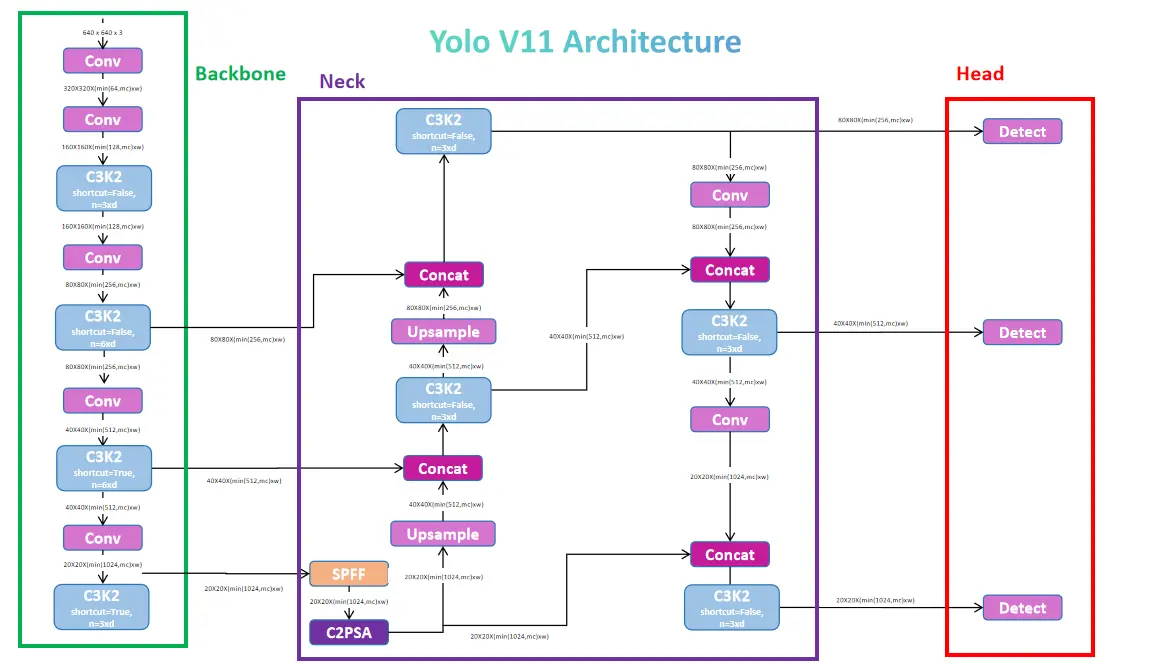
Diving into YOLOv11 Structure
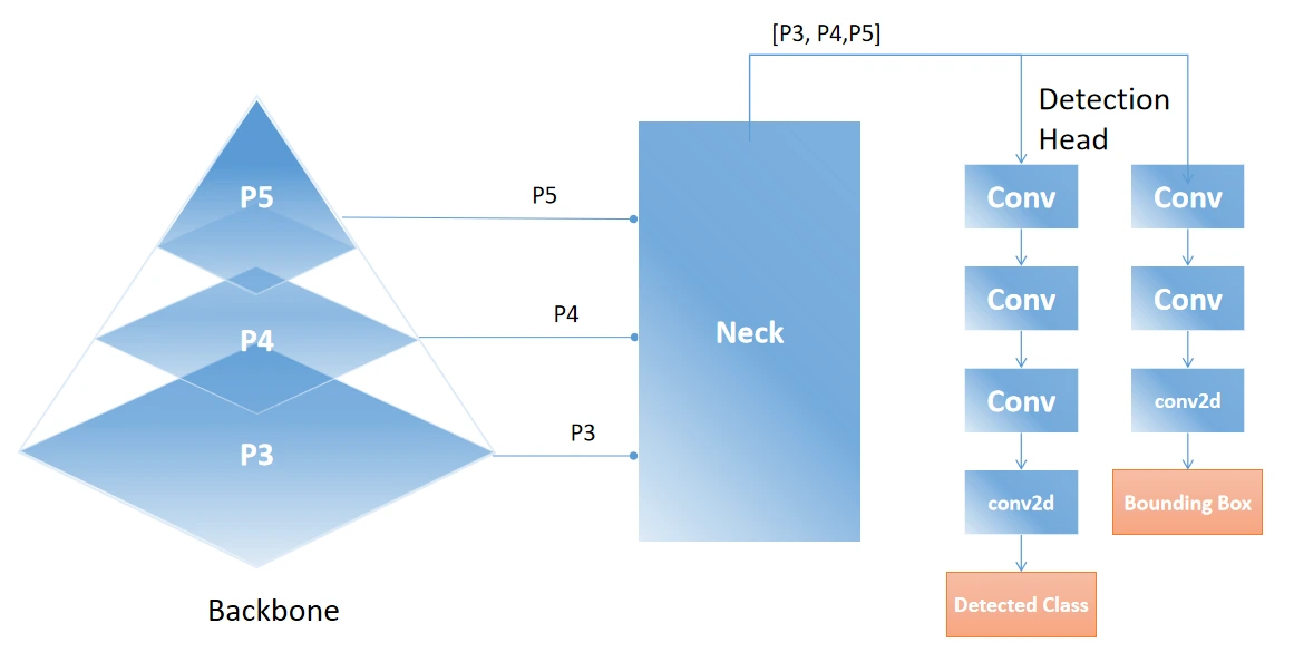
The YOLO fashions have a 3-section structure: spine, neck, and head. The spine extracts helpful options from the picture utilizing environment friendly bottleneck-based blocks. The neck processes the output from the spine and passes the options to the pinnacle. The pinnacle defines the duty of the mannequin, with choices like object detection, semantic segmentation, keypoint detection, picture classification, and oriented object detection. This part additionally makes use of convolution blocks, however they’re task-specific, which we’ll talk about intimately later.
YOLO Mannequin Capabilities
Beneath we’ll look into some most typical YOLO mannequin capabilities:
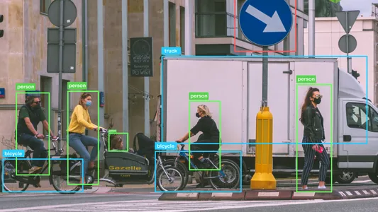
- Object Detection: Figuring out and finding objects inside a picture.
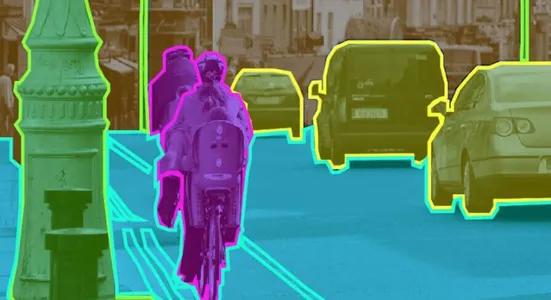
- Picture Segmentation: Detecting objects and delineating their boundaries.
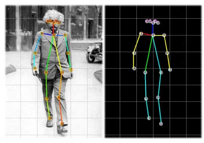
- Pose Estimation: Detecting and monitoring keypoints on human our bodies.
- Picture Classification: Categorizing photographs into predefined lessons.
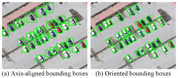
- Oriented Object Detection (OBB): Detecting objects with rotation for greater precision.
Exploring YOLOv11 Capabilities
The time period spine is often specified for the half the place the behind-the-scenes works are achieved. That’s what is going on within the Yolo fashions too. The primary process of any mannequin is to extract helpful options whereas contemplating parameters and velocity. The YoloV11 mannequin makes use of the DarkNet and DarkFPN spine, which is used to extract options. To get a greater understanding, assume the DarkNet mannequin is just like a CNN mannequin which is mostly used for classification or different duties, however by eradicating the final layers of the mannequin which assist generate the outputs, we modify the structure in such a means that, it will likely be helpful for function extraction.
The spine within the YOLO mannequin is used to extract 3 ranges of various options. Excessive-level options which are helpful for extracting data on detection options, semantic options, facial attributes, and many others. Medium-level options assist extract data on shapes, contours, ROIs, and patterns. Low-level options are helpful for detecting edges, shapes, textures, and gradients. The spine mannequin features a collection of convolutional and bottleneck blocks, together with a hybrid block known as C2K3, which mixes each varieties of blocks.
Core Parts of YOLOv11: Convolution and Bottleneck Layers
Beneath we’ll perceive the 2 most necessary layer:
Convolution Layer
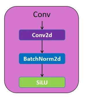
A convolutional layer is a part of a convolutional neural community (CNN) that extracts options from photographs. A batch normalization layer independently normalizes a mini-batch of information throughout all observations for every channel. The Convolution Block consists of a convolutional layer and a Batch Normalization layer earlier than passing it to the SiLU activation operate.
BottleNeck Layer
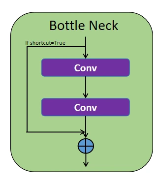
This block comprises two convolution blocks in collection with a concatenation operate. If the shortcut parameter is true, the enter is concatenated with the output from the second convolution block. If false, solely the output from the second block is handed by way of. This construction is principally utilized in blocks like C3K2 and SPFF, enhancing effectivity and enhancing studying.
Code Blocks
These are the utils codes :
# The autopad is used to detect the padding worth for the Convolution layer
def autopad(ok, p=None, d=1):
    if d > 1:
        # precise kernel-size
        ok = d * (ok - 1) + 1 if isinstance(ok, int) else [d * (x - 1) + 1 for x in k]
    if p is None:
        # auto-pad
        p = ok // 2 if isinstance(ok, int) else [x // 2 for x in k]
    return p

# That is the activation operate utilized in YOLOv11
class SiLU(nn.Module):
    @staticmethod
    def ahead(x):
        return x * torch.sigmoid(x)
Convolution Block (Con)
# The bottom Conv Block

class Conv(torch.nn.Module):

    def __init__(self, in_ch, out_ch, activation, ok=1, s=1, p=0, g=1):
        # in_ch = enter channels
        # out_ch = output channels
        # activation = the torch operate of the activation operate (SiLU or Identification)
        # ok = kernel measurement
        # s = stride
        # p = padding
        # g = teams
        tremendous().__init__()
        self.conv = torch.nn.Conv2d(in_ch, out_ch, ok, s, p, teams=g, bias=False)
        self.norm = torch.nn.BatchNorm2d(out_ch, eps=0.001, momentum=0.03)
        self.relu = activation

    def ahead(self, x):
        # Passing the enter by convolution layer and utilizing the activation operate
        # on the normalized output
        return self.relu(self.norm(self.conv(x)))

    def fuse_forward(self, x):
        return self.relu(self.conv(x))
Bottleneck Block
# The Bottlneck block

class Residual(torch.nn.Module):
    def __init__(self, ch, e=0.5):
        tremendous().__init__()
        self.conv1 = Conv(ch, int(ch * e), torch.nn.SiLU(), ok=3, p=1)
        self.conv2 = Conv(int(ch * e), ch, torch.nn.SiLU(), ok=3, p=1)

    def ahead(self, x):
        # The enter is handed by way of 2 Conv blocks and if the shortcut is true and
        # if enter and output channels are identical, then it's going to the enter as residual
        return x + self.conv2(self.conv1(x))
Now we you’ve got a short understanding of the essential blocks, let’s dive into the structure of the spine. YOLOv11 makes use of C3K2 blocks to deal with function extraction at completely different phases of the spine. The C3K2 block makes use of small-size kernels for environment friendly capturing of options. This block is an replace over the earlier present block C2F which is utilized in Yolov8.
C3K Module
# The C3k Module
class C3K(torch.nn.Module):
    def __init__(self, in_ch, out_ch):
        tremendous().__init__()
        self.conv1 = Conv(in_ch, out_ch // 2, torch.nn.SiLU())
        self.conv2 = Conv(in_ch, out_ch // 2, torch.nn.SiLU())
        self.conv3 = Conv(2 * (out_ch // 2), out_ch, torch.nn.SiLU())
        self.res_m = torch.nn.Sequential(Residual(out_ch // 2, e=1.0),
                                         Residual(out_ch // 2, e=1.0))

    def ahead(self, x):
        y = self.res_m(self.conv1(x)) # Course of half of the enter channels
        # Course of the opposite half instantly, Concatenate alongside the channel dimension
        return self.conv3(torch.cat((y, self.conv2(x)), dim=1))
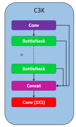
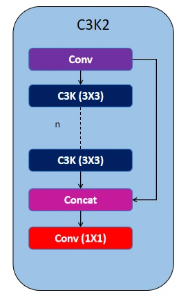
The C3K block consists of a Conv block adopted by a collection of bottleneck layers, with every layer’s options concatenated earlier than passing by way of the ultimate 1×1 Conv layer. Within the C3K2 block, a Conv block is used first, adopted by a collection of C3K blocks, after which handed to the 1×1 Conv block. This construction makes function extraction extra environment friendly in comparison with the earlier C2F block utilized in YOLOv8.
C3K2 Block Code
# The C3K2 Module

class C3K2(torch.nn.Module):
    def __init__(self, in_ch, out_ch, n, csp, r):
        tremendous().__init__()
        self.conv1 = Conv(in_ch, 2 * (out_ch // r), torch.nn.SiLU())
        self.conv2 = Conv((2 + n) * (out_ch // r), out_ch, torch.nn.SiLU())

        if not csp:
            # Utilizing the CSP Module when talked about True at shortcut
            self.res_m = torch.nn.ModuleList(Residual(out_ch // r) for _ in vary(n))
        else:
            # Utilizing the Bottlenecks when talked about False at shortcut
            self.res_m = torch.nn.ModuleList(C3K(out_ch // r, out_ch // r) for _ in vary(n))

    def ahead(self, x):
        y = checklist(self.conv1(x).chunk(2, 1))
        y.prolong(m(y[-1]) for m in self.res_m)
        return self.conv2(torch.cat(y, dim=1))
The spine mannequin structure begin with a Conv Block for the given picture enter of measurement 640 and three channels after which continues with 4 units of Conv Block with C3K2 Block. Then lastly use a Spatial Pyramid Pooling Quick (SPFF) Block.
Spatial Pyramid Pooling and Fusion (SPPF) Layer
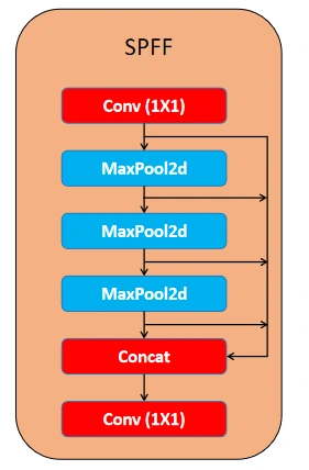
SPPF module (Spatial Pyramid Pooling Quick), which was designed to pool options from completely different areas of a picture at various scales. This improves the community’s skill to seize objects of various sizes, particularly small objects. It swimming pools options utilizing a number of max-pooling operations. The block comprises a 1X1 Conv Block adopted by a collection of MaxPool2D Layers with a concat block utilizing all of the residuals from the Maxpool2D layers, after which ending with a 1X1 Conv Block.
We extract three outputs (function maps) from the spine, akin to completely different ranges of granularity within the picture. This strategy helps detect small objects in finer element (P5) and bigger objects by way of higher-level options (P3). Low-level options come from the 2nd set of Conv Block and C3K2 Block. Medium-level options are from the third set, whereas higher-level options come from the 4th set. Due to this fact, for a given enter picture, the spine produces three outputs: P3, P4, and P5 in a listing.
Code Block for SPPF
# Code for SPFF Block
class SPPF(nn.Module):

    def __init__(self, c1, c2, ok=5):
        tremendous().__init__()
        c_          = c1 // 2
        self.cv1    = Conv(c1, c_, 1, 1)
        self.cv2    = Conv(c_ * 4, c2, 1, 1)
        self.m      = nn.MaxPool2d(kernel_size=ok, stride=1, padding=ok // 2)

    def ahead(self, x):
        x = self.cv1(x) # Beginning with a Conv Block
        y1 = self.m(x) # First MaxPool layer
        y2 = self.m(y1) # Second MaxPool layer
        return self.cv2(torch.cat((x, y1, y2, self.m(y2)), 1)) # Ending with Conv Block
Neural Community Neck: Characteristic Fusion and Transition Layer
Beneath part is a steady collection of blocks used to course of the extracted options from the block. Earlier than diving into the neck part, YOLOv11 additionally makes use of the C2PSA block. This block helps course of low-level objects by using the eye mechanism.
C2PSA
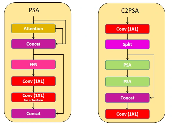
C2PSA refers to a Conv Block that makes use of two Partial Spatial Consideration (PSA) blocks. The PSA block combines Consideration, Conv, and FFNs to concentrate on the necessary objects within the function map given to it, and the modified model of PSA is C2PSA. This block begins with a 1×1 Conv Block, then splits the function map in half, sequentially making use of two PSA blocks. A concat block provides the output of the second PSA block to the unprocessed cut up, and the block ends with one other 1×1 Conv block. This structure helps to course of the function maps in separate branches, and later concatenate. This ensures the mannequin focuses on data, computational value and accuracy concurrently.
Code for Consideration Module
The code defines an Consideration module that makes use of multi-head consideration. It initializes parts like question, key, and worth (QKV) layers and processes enter by way of convolution layers. Within the ahead methodology, the enter is cut up into queries, keys, and values, and a spotlight scores are computed. The output is a weighted sum of the values, refined by way of further convolution layers, enhancing function illustration and capturing spatial dependencies.
# Code for the Consideration Module

class Consideration(torch.nn.Module):

    def __init__(self, ch, num_head):
        tremendous().__init__()
        self.num_head = num_head
        self.dim_head = ch // num_head
        self.dim_key = self.dim_head // 2
        self.scale = self.dim_key ** -0.5

        self.qkv = Conv(ch, ch + self.dim_key * num_head * 2, torch.nn.Identification())

        self.conv1 = Conv(ch, ch, torch.nn.Identification(), ok=3, p=1, g=ch)
        self.conv2 = Conv(ch, ch, torch.nn.Identification())

    def ahead(self, x):
        b, c, h, w = x.form

        qkv = self.qkv(x)
        qkv = qkv.view(b, self.num_head, self.dim_key * 2 + self.dim_head, h * w)

        q, ok, v = qkv.cut up([self.dim_key, self.dim_key, self.dim_head], dim=2)

        attn = (q.transpose(-2, -1) @ ok) * self.scale
        attn = attn.softmax(dim=-1)

        x = (v @ attn.transpose(-2, -1)).view(b, c, h, w) + self.conv1(v.reshape(b, c, h, w))
        return self.conv2(x)
Code for PSAModule
The PSABlock module combines consideration and convolutional layers to boost function illustration. It first applies an consideration module to seize dependencies, then processes the output by way of two convolution blocks. The ultimate output combines the unique enter and the processed options, enhancing data circulate and studying.
# Code for the PSAModule
class PSABlock(torch.nn.Module):
    # This Module has a sequential of 1 Consideration module and a couple of Conv Blocks
    def __init__(self, ch, num_head):
        tremendous().__init__()
        self.conv1 = Consideration(ch, num_head)
        self.conv2 = torch.nn.Sequential(Conv(ch, ch * 2, torch.nn.SiLU()),
                                         Conv(ch * 2, ch, torch.nn.Identification()))

    def ahead(self, x):
        x = x + self.conv1(x)
        return x + self.conv2(x)
Code for C2PSA
Coming again to the neck half, additionally it is part of the options extraction and this primarily focuses on options processing. The neck half processes the three ranges of options, every with completely different channel sizes. To deal with this, the mannequin adjusts all of the channels to the identical quantity after which extracts them utilizing intermediate layers. Let’s go within the element.
Implementation
# PSA Block Code

class PSA(torch.nn.Module):

    def __init__(self, ch, n):
        tremendous().__init__()
        self.conv1 = Conv(ch, 2 * (ch // 2), torch.nn.SiLU())
        self.conv2 = Conv(2 * (ch // 2), ch, torch.nn.SiLU())
        self.res_m = torch.nn.Sequential(*(PSABlock(ch // 2, ch // 128) for _ in vary(n)))

    def ahead(self, x):
        # Passing the enter to the Conv Block and splitting into two function maps
        x, y = self.conv1(x).chunk(2, 1)
        # 'n' variety of PSABlocks are made sequential, after which passes one them (y) of
        # the function maps and concatenate with the remaining function map (x)
        return self.conv2(torch.cat(tensors=(x, self.res_m(y)), dim=1))
The low-level options (P5) are of form 20X20X1024, the medium-level options (P4) are of form 40X40X512 and the high-level options (P5) are of form 80X80X256. We first cross the low-level options (output of SPFF) to C2PSA, which outputs attention-based options targeted on spatial data. We then upsample the output to the form of P4 and concatenate it with P4 options. Subsequent, we upsample the mixed options to the form of P3 and concatenate them with P3 options. This course of upscales and concatenates all of the options. Lastly, we ship the options to the C3K2 block to course of them higher utilizing the Bottlenecks.
We identify the output of the C3K2 block as feat1, which represents the high-level options that can be despatched to the pinnacle part. We downsample feat1, concatenate it with P4, and ship it to the C3K2 block. The output, feat2, consists of the medium-level options that can be despatched to the pinnacle part. We repeat the identical course of with the low-level options, concatenate them with P5 (output of C2PSA), and ship them to the C3K2 block. The output, feat3, represents the low-level options despatched to the pinnacle part.
We are going to code the neck half eventually together with the pinnacle half.
The pinnacle part can have a listing of three outputs containing feat1, feat2, and feat3. Let’s discover the Head part and see how the three options are used for duties like Object Detection, Segmentation, and Keypoint Detection.
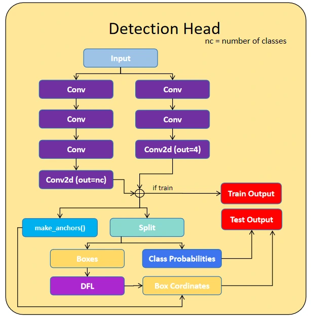
Understanding The Head
YOLO mannequin makes use of three process heads: the Detection Head, Segmentation Head, and Keypoint Detection Head.
The primary head is the Detection Head, which makes use of three options for DFL (Focal Loss), Field Detection, and Class Detection. The DFL block calculates the focal loss, whereas the Field Detection consists of sequential convolution layers that output a form of 4, representing the coordinates of the field. Class Detection additionally makes use of sequential layers of the convolutional layer to course of the options utilizing the SiLU activation operate and output of a single class and later handed with the sigmoid operate to get a one-hot encoding output.
DFL Perform Code
class DFL(nn.Module):
    # Distribution Focal Loss (DFL) proposed in Generalized Focal Loss https://ieeexplore.ieee.org/doc/9792391
    def __init__(self, c1=16):
        tremendous().__init__()
        self.conv   = nn.Conv2d(c1, 1, 1, bias=False).requires_grad_(False)
        x           = torch.arange(c1, dtype=torch.float)
        self.conv.weight.knowledge[:] = nn.Parameter(x.view(1, c1, 1, 1))
        self.c1     = c1

    def ahead(self, x):
        b, c, a = x.form
        return self.conv(x.view(b, 4, self.c1, a).transpose(2, 1).softmax(1)).view(b, 4, a)
The segmentation and key level detection used this Detection block as their mother or father class and processed their output based on their shapes, segmentation outputs the form equal to the picture form and the important thing level detection outputs the form of [17,3] or [17,2] primarily based on the requirement. The important thing factors are usually 17 key factors for the particular person 2 are the x and y coordinated 17 are the places within the particular person, 3 are the x and y coordinated and one other variable indicating it’s for the visibility of key level functions.
Yolo Mannequin Variations
We all know that there are 5 variations of the YOLO mannequin, i.e., nano (n), small (s), medium (m), giant (l), and further giant (x). The primary distinction between these variations is the sizes of the function maps they course of. The function map shapes can decided utilizing the spine output shapes, for the nano variations the output function map shapes are 40x40x64, 20x20x128 and 20x20x256, for the small model we get the shapes, 40x40x128, 20x20x256 and 20x20x512.
We have to obtain the dynamic channel setting, to get this drawback solved we set depth and width whereas defining the mannequin and in addition point out when to make use of the C3K Modules for use within the C3K2 block as a listing of boolean values. These three inputs to the primary mannequin operate could make 5 variations of the YOLO mannequin from nano to additional giant. The depth is used within the spine to repeat the variety of C3K modules and the width represents the picture decision.
Full YOLOv11 Mannequin: Spine, Neck and Head
Let’s concentrate on the Object Detection process and Let’s Code the whole Yolo Mannequin.
The Spine
class DarkNet(torch.nn.Module):
    def __init__(self, width, depth, csp):
        tremendous().__init__()
        self.p1 = []
        self.p2 = []
        self.p3 = []
        self.p4 = []
        self.p5 = []

        # p1/2
        self.p1.append(Conv(width[0], width[1], torch.nn.SiLU(), ok=3, s=2, p=1))
        # p2/4
        self.p2.append(Conv(width[1], width[2], torch.nn.SiLU(), ok=3, s=2, p=1))
        self.p2.append(CSP(width[2], width[3], depth[0], csp[0], r=4))
        # p3/8
        self.p3.append(Conv(width[3], width[3], torch.nn.SiLU(), ok=3, s=2, p=1))
        self.p3.append(CSP(width[3], width[4], depth[1], csp[0], r=4))
        # p4/16
        self.p4.append(Conv(width[4], width[4], torch.nn.SiLU(), ok=3, s=2, p=1))
        self.p4.append(CSP(width[4], width[4], depth[2], csp[1], r=2))
        # p5/32
        self.p5.append(Conv(width[4], width[5], torch.nn.SiLU(), ok=3, s=2, p=1))
        self.p5.append(CSP(width[5], width[5], depth[3], csp[1], r=2))
        self.p5.append(SPP(width[5], width[5]))
        self.p5.append(PSA(width[5], depth[4]))

        self.p1 = torch.nn.Sequential(*self.p1)
        self.p2 = torch.nn.Sequential(*self.p2)
        self.p3 = torch.nn.Sequential(*self.p3)
        self.p4 = torch.nn.Sequential(*self.p4)
        self.p5 = torch.nn.Sequential(*self.p5)

    def ahead(self, x):
        p1 = self.p1(x)
        p2 = self.p2(p1)
        p3 = self.p3(p2)
        p4 = self.p4(p3)
        p5 = self.p5(p4)
        return p3, p4, p5
The Neck
class DarkFPN(torch.nn.Module):
    def __init__(self, width, depth, csp):
        tremendous().__init__()
        self.up = torch.nn.Upsample(scale_factor=2)
        self.h1 = CSP(width[4] + width[5], width[4], depth[5], csp[0], r=2)
        self.h2 = CSP(width[4] + width[4], width[3], depth[5], csp[0], r=2)
        self.h3 = Conv(width[3], width[3], torch.nn.SiLU(), ok=3, s=2, p=1)
        self.h4 = CSP(width[3] + width[4], width[4], depth[5], csp[0], r=2)
        self.h5 = Conv(width[4], width[4], torch.nn.SiLU(), ok=3, s=2, p=1)
        self.h6 = CSP(width[4] + width[5], width[5], depth[5], csp[1], r=2)

    def ahead(self, x):
        p3, p4, p5 = x
        p4 = self.h1(torch.cat(tensors=[self.up(p5), p4], dim=1))
        p3 = self.h2(torch.cat(tensors=[self.up(p4), p3], dim=1))
        p4 = self.h4(torch.cat(tensors=[self.h3(p3), p4], dim=1))
        p5 = self.h6(torch.cat(tensors=[self.h5(p4), p5], dim=1))
        return p3, p4, p5
The Head
The make_anchors operate generates anchor factors and their corresponding strides for object detection. It processes function maps at completely different scales, making a grid of anchor coordinates (centre factors) with an optionally available offset for alignment. The operate outputs tensors of anchor factors and strides, that are essential for outlining areas in object detection duties the place bounding containers are predicted.
def make_anchors(x, strides, offset=0.5):
    assert x will not be None
    anchor_tensor, stride_tensor = [], []
    dtype, machine = x[0].dtype, x[0].machine
    for i, stride in enumerate(strides):
        _, _, h, w = x[i].form
        sx = torch.arange(finish=w, machine=machine, dtype=dtype) + offset  # shift x
        sy = torch.arange(finish=h, machine=machine, dtype=dtype) + offset  # shift y
        sy, sx = torch.meshgrid(sy, sx)
        anchor_tensor.append(torch.stack((sx, sy), -1).view(-1, 2))
        stride_tensor.append(torch.full((h * w, 1), stride, dtype=dtype, machine=machine))
    return torch.cat(anchor_tensor), torch.cat(stride_tensor)
The fuse_conv operate merges a convolution layer (conv) and a normalization layer (norm) right into a single convolution layer by adjusting its weights and biases. That is generally used throughout mannequin optimization for deployment, because it removes the necessity for separate normalization layers, enhancing inference velocity and lowering reminiscence utilization with out altering the mannequin’s behaviour.
def fuse_conv(conv, norm):
    fused_conv = torch.nn.Conv2d(conv.in_channels,
                                 conv.out_channels,
                                 kernel_size=conv.kernel_size,
                                 stride=conv.stride,
                                 padding=conv.padding,
                                 teams=conv.teams,
                                 bias=True).requires_grad_(False).to(conv.weight.machine)

    w_conv = conv.weight.clone().view(conv.out_channels, -1)
    w_norm = torch.diag(norm.weight.div(torch.sqrt(norm.eps + norm.running_var)))
    fused_conv.weight.copy_(torch.mm(w_norm, w_conv).view(fused_conv.weight.measurement()))

    b_conv = torch.zeros(conv.weight.measurement(0), machine=conv.weight.machine) if conv.bias is None else conv.bias
    b_norm = norm.bias - norm.weight.mul(norm.running_mean).div(torch.sqrt(norm.running_var + norm.eps))
    fused_conv.bias.copy_(torch.mm(w_norm, b_conv.reshape(-1, 1)).reshape(-1) + b_norm)

    return fused_conv
The Object Detection Head
class Head(torch.nn.Module):
    anchors = torch.empty(0)
    strides = torch.empty(0)

    def __init__(self, nc=80, filters=()):
        tremendous().__init__()
        self.ch = 16  # DFL channels
        self.nc = nc  # variety of lessons
        self.nl = len(filters)  # variety of detection layers
        self.no = nc + self.ch * 4  # variety of outputs per anchor
        self.stride = torch.zeros(self.nl)  # strides computed throughout construct

        field = max(64, filters[0] // 4)
        cls = max(80, filters[0], self.nc)

        self.dfl = DFL(self.ch)

        self.field = torch.nn.ModuleList(
           torch.nn.Sequential(Conv(x, field,torch.nn.SiLU(), ok=3, p=1),
           Conv(field, field,torch.nn.SiLU(), ok=3, p=1),
           torch.nn.Conv2d(field, out_channels=4 * self.ch,kernel_size=1)) for x in filters)

        self.cls = torch.nn.ModuleList(
            torch.nn.Sequential(Conv(x, x, torch.nn.SiLU(), ok=3, p=1, g=x),
            Conv(x, cls, torch.nn.SiLU()),
            Conv(cls, cls, torch.nn.SiLU(), ok=3, p=1, g=cls),
            Conv(cls, cls, torch.nn.SiLU()),
            torch.nn.Conv2d(cls, out_channels=self.nc,kernel_size=1)) for x in filters)

    def ahead(self, x):
        for i, (field, cls) in enumerate(zip(self.field, self.cls)):
            x[i] = torch.cat(tensors=(field(x[i]), cls(x[i])), dim=1)
        if self.coaching:
            return x

        self.anchors, self.strides = (i.transpose(0, 1) for i in make_anchors(x, self.stride))
        x = torch.cat([i.view(x[0].form[0], self.no, -1) for i in x], dim=2)
        field, cls = x.cut up(split_size=(4 * self.ch, self.nc), dim=1)

        a, b = self.dfl(field).chunk(2, 1)
        a = self.anchors.unsqueeze(0) - a
        b = self.anchors.unsqueeze(0) + b
        field = torch.cat(tensors=((a + b) / 2, b - a), dim=1)

        return torch.cat(tensors=(field * self.strides, cls.sigmoid()), dim=1)
Defining the YOLOv11 Mannequin
class YOLO(torch.nn.Module):
    def __init__(self, width, depth, csp, num_classes):
        tremendous().__init__()
        self.internet = DarkNet(width, depth, csp)
        self.fpn = DarkFPN(width, depth, csp)

        img_dummy = torch.zeros(1, width[0], 256, 256)
        self.head = Head(num_classes, (width[3], width[4], width[5]))
        self.head.stride = torch.tensor([256 / x.shape[-2] for x in self.ahead(img_dummy)])
        self.stride = self.head.stride
        self.head.initialize_biases()

    def ahead(self, x):
        x = self.internet(x)
        x = self.fpn(x)
        return self.head(checklist(x))

    def fuse(self):
        for m in self.modules():
            if sort(m) is Conv and hasattr(m, 'norm'):
                m.conv = fuse_conv(m.conv, m.norm)
                m.ahead = m.fuse_forward
                delattr(m, 'norm')
        return self
Defining Totally different Variations of YOLOv11 Fashions
class YOLOv11:
  def __init__(self):

    self.dynamic_weighting = {
      'n':{'csp': [False, True], 'depth' : [1, 1, 1, 1, 1, 1], 'width' : [3, 16, 32, 64, 128, 256]},
      's':{'csp': [False, True], 'depth' : [1, 1, 1, 1, 1, 1], 'width' : [3, 32, 64, 128, 256, 512]},
      'm':{'csp': [True, True], 'depth' : [1, 1, 1, 1, 1, 1], 'width' : [3, 64, 128, 256, 512, 512]},
      'l':{'csp': [True, True], 'depth' : [2, 2, 2, 2, 2, 2], 'width' : [3, 64, 128, 256, 512, 512]},
      'x':{'csp': [True, True], 'depth' : [2, 2, 2, 2, 2, 2], 'width' : [3, 96, 192, 384, 768, 768]},
    }
  def build_model(self, model, num_classes):
    csp = self.dynamic_weighting[version]['csp']
    depth = self.dynamic_weighting[version]['depth']
    width = self.dynamic_weighting[version]['width']
    return YOLO(width, depth, csp, num_classes)
Evaluation of Mannequin
Now that now we have outlined our mannequin, we should verify whether or not all of the code blocks and the entire mannequin structure are appropriately designed. To do that, we have to outline the mannequin, verify for the mannequin parameters, and cross-check with the official parameter depend given. This methodology permits us to substantiate that the mannequin structure is constructed appropriately. To do that, we have to set up a library named thop.
GFLOPS : (Giga Floating-Level Operations Per Second)
This metric measures a mannequin’s computation efficiency, notably in laptop imaginative and prescient. It represents the variety of floating-point operations carried out per second. It’s crucial to verify the use case and the connection between the mannequin and the respective {hardware}. A better GFLOPS worth usually signifies quicker processing, enabling real-time efficiency and supporting advanced fashions in functions equivalent to autonomous automobiles and medical imaging.
Checking the GLOPS
We are able to use the profile operate from thop library to verify the GLOPS and parameters depend. First, we have to outline a random tensor of 3 channel picture of measurement 640. The enter tensor form must be within the dimension of (batch measurement, variety of channels, width, top). We declare this enter retailer it within the dummy_input variable, and initialize the mannequin of the nano model with 80 lessons. Then we give the mannequin, dummy_input to the profile operate and it returns the FLOPS and Parameters. Then we print the FLOPS in Giga varieties, representing it as GLOPS and the parameter depend of the mannequin. Via this course of, we decide the GLOPS and Parameter depend utilizing the thop library.
!pip set up thop

from thop.profile import profile

dummy_input = torch.randn(1, 3, 640, 640)

mannequin = YOLOv11().build_model(model='n', num_classes=80)
flops, params = profile(mannequin, (dummy_input,), verbose=False)

print(f"Params: {params / 1e6:.3f}M")
print(f"GFLOPs: {flops / 1e9:.3f}")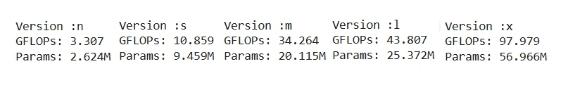
These are the mannequin parameters that now we have obtained they usually match with the official parameters depend given by the Ultralytics, Therefore our mannequin constructing is appropriate! Supply
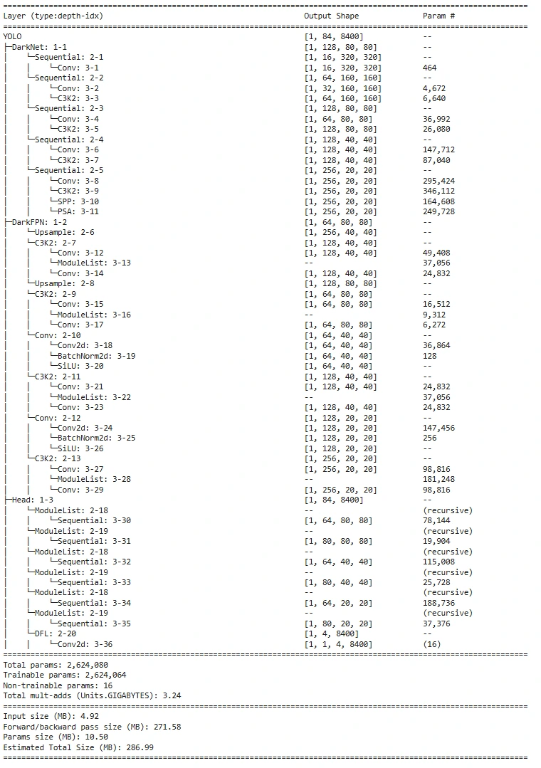
Mannequin Structure
To investigate the mannequin structure and decide, indicating every layer and its output form of the function map, we use the torchinfo library to indicate the mannequin structure with parameters depend. This is named mannequin abstract, additionally we can be going to import the operate named abstract from the torchinfo. This operate takes enter from the mannequin and in addition the input_data to showcase the mannequin abstract, and input_data is optionally available. Right here is the code to print the mannequin abstract utilizing the torchinfo library.
!pip set up torchinfo

import torch
from torchinfo import abstract


# Figuring out the machine through which the present env is working
machine = torch.machine("cuda" if torch.cuda.is_available() else "cpu")


# Creating enter tensor and transferring it to the machine
dummy_input = torch.randn(1, 3, 640, 640).to(machine)

# Creating the mannequin and transferring it to the machine
mannequin = YOLOv11().build_model(model='n', num_classes=80).to(machine)

# Now run the abstract operate from torchinfo
abstract(mannequin, input_data=dummy_input)
The output you get for the nano model
Yeah! You’ve realized tips on how to construct a mannequin from scratch by understanding its fundamentals. Nonetheless, the work of an actual laptop imaginative and prescient engineer is way from over. The following step is writing the practice and take a look at code for datasets in COCO or YOLO format. For these concerned about testing the mannequin, let’s dive into tips on how to print the output for a random tensor.
Testing the Mannequin with random enter tensor
As an alternative of taking a significant picture, let’s use a random torch tensor for experimental and understanding functions. We give the tensor’s mannequin enter after which look at the mannequin output.
# the dummy enter of random values
dummy_input = torch.randn(1, 3, 640, 640)

# defining the mannequin of nano model
mannequin = YOLOv11().build_model(model='n', num_classes=80)

# lets print the output
output = mannequin(dummy_input)

print(f"Sort of the output :{sort(output)}, Size of the output: {len(output)}")
print(f"The shapes every output function map : {output[0].form, output[2].form, output[2].form}")
By this code, you see that the output from the mannequin isn’t the anticipated bounding field and sophistication, however as a substitute, we’re getting the three pyramid function maps output. As a result of the mannequin is defaulted in practice mode, these function maps would be the output when the mannequin is in practice mode. Let’s see what’s the output in eval mode.
# Transfer the mannequin to eval mannequin
mannequin.eval()
eval_output = mannequin(dummy_input)

# Let' see what are the outputs
print(f"Output form: {eval_output.form}")

# Anticipated consequence : torch.Measurement([1, 84, 8400])
The output here’s a torch tensor of form [1,84,8400]. Right here 1 is the batch measurement of the enter, and 84 is the variety of outputs per anchor. It consists of 4 values for the bounding field and 80 class possibilities and 8400 is the entire variety of anchors/predictions. From this, we’ll use an idea named Non-Most Suppression (NMS) which is a method utilized in object detection to get rid of redundant bounding containers for a similar object. It really works by rating predictions primarily based on their confidence scores and iteratively deciding on the highest-scoring field whereas suppressing others with vital overlap past a predefined threshold. This ensures that solely probably the most related and non-overlapping detections are retained, enhancing the readability and precision of the output. We are going to get again to this idea within the subsequent article.
What’s Subsequent?
In case you are considering that now we have constructed the mannequin and know tips on how to course of the output too, then what’s subsequent? The following process is expounded to dataset processing, coaching and validation knowledge loader, coaching code and testing code with efficiency metrics calculation. All matters can be fully lined within the upcoming article, so keep tuned on Analytics Vidhya.
Conclusion
YOLOv11 continues the legacy of the YOLO household by introducing an optimized structure that balances accuracy, velocity, and effectivity. With its superior spine, neck, and head parts, the mannequin excels in duties like object detection, segmentation, and pose estimation. Its sensible, application-driven design makes it a robust device for real-world AI options, pushing the boundaries of deep learning-based detection fashions.
Key Takeaways
- YOLOv11 builds on earlier YOLO variations with an enhanced spine and have extraction methods.
- It helps a number of duties, together with object detection, segmentation, and classification.
- The mannequin’s structure emphasizes effectivity with C3K and C3K2 modules for improved function studying.
- YOLOv11 prioritizes real-world functions over conventional analysis documentation.
- Its optimized design makes it appropriate for deployment in edge and high-performance computing environments.
The media proven on this article will not be owned by Analytics Vidhya and is used on the Creator’s discretion.
I’m Nikhileswara Rao Sulake, a DRDO and DIAT licensed AI Skilled from Andhra Pradesh. I’m an AI practitioner working within the area of Deep Studying and Pc Imaginative and prescient. I’m proficient in ML, DL, CV, NLP and AR applied sciences. I’m presently engaged on analysis papers on Deep Studying and Pc Imaginative and prescient.